Bits

Binary digits (1s and 0s) are the atoms of the computer science universe because every piece of code ultimately translates into a sequence of 1s and 0s which we feed into the computer. This sequence tells the computer exactly what to do to make our program work. We refer to these binary digits as “bits”.¹

Functional Completeness

Before we dive into how this process of how running a chunk of binary code works, let’s first understand why we are able to translate everything into a sequence of bits. Consider the fact that we can describe every program as a set of instructions, which are simply sentences made up of words. Let’s call this set of all English words A.

This set A is \df{functionally complete}, meaning we can describe any program or function using only elements in this set.² Now, we can \df{map} each word in A to an integer—to map simply means to assign each element in A a corresponding element in our set of positive integers, denoted \mathbb{Z}^+. For example, if we were to go through a dictionary mapping words to consecutive numbers, the first word maps to 1, the second maps to 2, and so on.

According to Wikipedia, there are 588,632 English words (as of writing this), so our set of integers would go from 1 all the way up to 588,632. Therefore, this set of integers, call it B, is also functionally complete if we say the integers translate to the words. Essentially, we’ve created a set A whose elements can describe any program.

Now we will map this set of integers to a set C of binary strings (meaning sequences of bits), proving that C is also functionally complete—in other words, every function can be created using only strings of bits, which correspond to English words.

An inefficient way to do this would be to map every integer to its corresponding number of 1’s: for example, 3\rightarrow 111, 4\rightarrow 1111, and so on. This method works, but is inefficient because it requires 588,632 bits! Let’s look at a better way of doing this.

The 17th century mathematician Gottfried Wilhelm Leibniz discovered that integers in base 10 (decimal) can be represented in base 2 (binary) using a string of 1’s and 0’s corresponding to the powers of 2. In a binary string of n bits, this conversion to decimal takes the form of b_{n-1}2^{n-1}+b_{n-2}2^{n-2}+\dots+b_02^0. For example, if we have a binary string of length 4, b_3b_2b_1b_0 (meaning each b_n is either a 1 or a 0), the corresponding integer in base-10 is equal to b_32^3 + b_2 2^2 + b_1 2^1 + b_0 2^0=8b_3+4b_2+2b_1+b_0.

Using n bits we can represent positive integers in the range \eqlabel{binary range}{1} [0,2^{n}). Note that the right bound is exclusive, meaning that the bound includes integers up to, but not including 2^n. Therefore, we can represent integers from 0 to 2^n-1. In the case where n=4, we can represent numbers in the range [0,2^{n})=[0,32). To represent a number in binary, think of your decimal number n as having n units. In the binary string, each bit b_i holds 2^i units. We place a 1 at the largest bit b_i whose value, 2^i, is less than or equal to n. Then incrementally go left to right, filling up the remaining n-2^i units of our number, at each bit subtracting the units we fill up until we are left with 0 units.

Let’s look at the example of representing 13 in binary. The largest power of 2 less than or equal to 13 is 2^3=8, then the largest power of 2 less than or equal to 13-8=5 is 2^2=4, then finally the largest power of 2 less than or equal to 5-4=1 is 2^0=1. Now we have finished because we are left with 1-1=0 units. We place a 1 at the bit corresponding to each power of 2 we used, and a zero otherwise. This yields the binary string 1101: 1(2^3)+1(2^2)+0(2^1)+1(2^0)=8+4+0+1=13

Now returning to our idea of functional completeness with sets A of words, B of positive integers, and C of binary strings, let’s use this new method of mapping our set of integers B to binary strings C. Figure \ref{#fig:mapping}{2} illustrates the mapping obtained using binary strings of 20 bits.

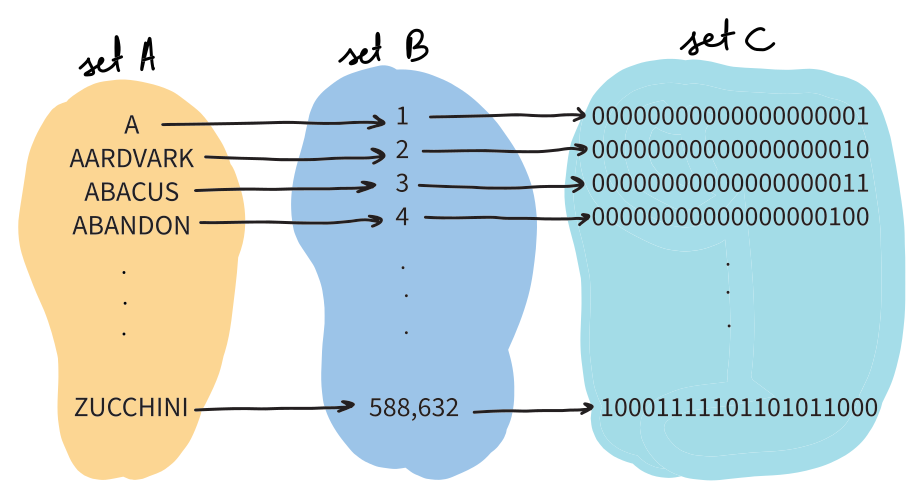
Why 20 bits? Because 20 is the minimum number of bits we can use to represent our range of integers from 1 to 588,632 in set B: \begin{array}{r c l} \ceil{2^n-1} & = & 588,632 \\ \ceil{2^n} & = & 588,633 \\ n & = & \ceil{\log_2(588,633)}=\ceil{19.167}=20 \end{array} In the above expression, the ceiling function, ceil(x)=\ceil{x}, rounds x up to the nearest integer. On the other hand, the floor function, floor(x)=\floor{x} rounds x down to the nearest integer.

Therefore, we could describe any function by stringing together these 20-bit chunks—which map to English words—as we would when constructing a sentence. However, 588,632 words is far more than necessary for describing functions, and in fact the intel x86 processors use only 81 \df{opcodes} (a fancy word for computer chip instructions) to run all of the programs we use today!

Each instruction requires a hard-coded circuit, so having 588,632 of these would be far too much. We’ll expand upon opcodes more once we start learning about programming in the assembly coding language.

New Forms of Counting

So how did Leibniz formulate this system of binary counting? Well, let’s examine the form of counting which we are more familiar with—base 10, also known as decimal. We call it base 10 because the way in which we count is rooted in the powers of 10.

As an example, let’s consider the number 430. What does this number mean? Well, it is equivalent to the expression 4(10^2)+3(10^1)+0(10^0)=400+30+0. Our digits, which are coefficients of the powers of 10, lie in the range [0,10). We can assign each digit a variable d_i where i is the digit’s position in our expression. This yields the following assignments: d_2=4, d_1=3, and d_0=0.

When digit i, d_i, becomes greater than or equal to 10, we divide d_i by 10 rounding down and sum the result with the next greatest coefficient, d_{i+1}: d_{i+1}+=\floor{d_i/10}. We then set d_i to the remainder of the operation. We call this operation of obtaining the remainder \df{modulo}, denoted by \%. Equation \eqref{#modulo}{2} shows the equivalent algebraic expression for modulo: \eqlabel{modulo}{2} d_i\%10=d_i-10\floor{d_i/10} This is just a fancy way of saying we carry the 1, as shown in figure \ref{#fig:carry 1}{3}.

\begin{array}{ccc} & \textcolor{blue}{\mathbf{{}^1}} &\\ & 2 & 5\\ + & 3 & 7\\ \hline & 6 & 2 \end{array}

In general, we can represent all non-negative integers in a base-n counting system using the form

x_i(n^i)+x_{i-1}(n^{i-1})+\dots+x_0(n^0) where each x lies in the range [0,n) and n is a positive integer. This is incredibly powerful because we can represent the same information in different ways! We will see in the next section how this new form of counting allows us to store information in a computer, more specifically, how the binary counting system tailors to the simple architecture of a microprocessor’s transistor.

A popular form of counting in computer science is base-16, also known as \df{hexadecimal}. To store d values greater than 9, we use English letters A to F for representing digit-values 10 to 15. Also, we add on the prefix ‘0x’ to hexadecimal values to distinguish them from base-10 decimal values. See table \ref{#base comparison}{4} for a side-by-side comparison of counting in binary, decimal, and hexadecimal.

Base-2	Base-10	Base-16
0	0	0x0
1	1	0x1
10	2	0x2
11	3	0x3
100	4	0x4
101	5	0x5
110	6	0x6
111	7	0x7
1000	8	0x8
1001	9	0x9
1010	10	0xA
1011	11	0xB
1100	12	0xC
1101	13	0xD
1110	14	0xE
1111	15	0xF
10000	16	0x10

When we talk about values stored in the computer’s memory, we typically use hexadecimal (base-16) because it is a multiple of binary (base-2), but easier to read due to its compact form (e.g. 0xE8 vs. 11101000). Computers process information in groups of 8 bits, also known as \df{bytes}, so two hex values represents one byte.

Figure \ref{#fig:counting}{5} provides another lens we can use to view counting in binary, decimal, and hexadecimal. After every column of digit d_i is filled up, the squares units in d_i plus one unit equals one column in the next digit, d_{i+1}. Therefore, if d_i is full and we add one more column to d_i, we carry over all of the units in d_i to fill up a single column in d_{i+1}, and we are left with an empty d_i.

Let’s say we are counting in base-n. If we have x columns filled in d_i, we fill \floor{x/n} columns of d_{i+1} and we are left with x\%n columns filled in d_i. This is just the fancy mathematical way of saying that we transfer as many columns that we can fill of the next digit from the current.

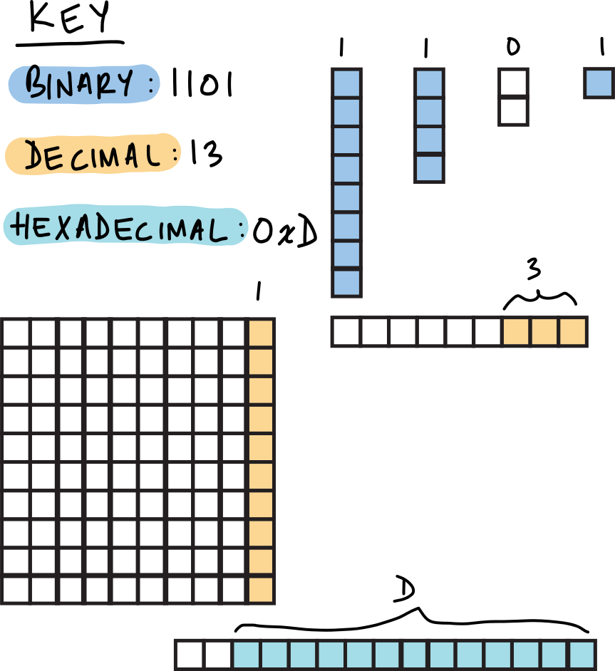
Think about the different forms of counting as a trade-off between how many digits we use to represent a number (the number columns in figure \ref{#fig:counting}{5}) and how fast the buckets corresponding to our digits grow as we add on the next digit (the number of rows in figure \ref{#fig:counting}{5}). We can hold more information with larger buckets, e.g. two digits in decimal can store the range [0,10^2) whereas two digits in binary can only store the range [0,2^2). However, we need n unique characters to map to each of the digit’s n states. Once we go past base 36, we run out of numbers 0 to 9 and letters A to Z.³

Now that we know there are an infinite number of ways to count by using different bases, let’s examine why computers count in base-2 and how this tailors to the simple architecture of the microprocessor’s \df{transistor}.⁴

Holding State: on/off

Computers operate in binary because at the microscopic level it is easiest to deal with measuring only two states: on or off. Central Processing Units (CPUs) contain millions of transistors, which measure voltage passing through them and hold a state value of 0 or 1. Think of a transistor as a light switch that can either be on or off. Its state is assigned based on whether the voltage passing surpasses 0.7V:

\begin{cases} voltage<0.7V & 0, \text{transistor is off} \\ voltage\ge0.7V & 1, \text{transistor is on} \end{cases}

Adding another voltage threshold to allow transistors to take on three state values could lead to inaccuracies in calculating state due to there being less room for error in voltage checks—we can only pass so much voltage through a 5 nanometer transistor! Furthermore, this added threshold would only be a duplication of the current transistor architecture, so it makes sense to stick with only one threshold and thereby two states for transistors.

In the case of quantum computers, the foundational building block is a \df{qubit}, which stores information not through an on/off voltage threshold, but rather through the spin of an electron. The qubit can take on an infinite number of states because there is an infinite number of ways to spin an electron in 3 dimensional space. However, due to quantum physics, once you measure a qubit’s value it takes on one of two states with a probability corresponding to the electron’s last spin. Therefore, we make quantum calculations by having the qubits interact with each other and undergo spin changes, then we measure the result at the end. Nature does all the work!

You can think about using bits as counting information in base 2 and using qubits as counting in base infinity—that is, until you measure the qubit. Now that we have a better understanding of the hardware reasons for why computers operate in base 2 as well as how counting in binary works, we will now examine the hardware implementation of a transistor.

How Does a Transistor Work?

We know that transistors turn on and off like a light switch, but rather than flicking a physical switch, we apply voltage to change the transistor’s state. To fully understand how a transistor works we need to look at its design at an atomic level.

Silicon is the element of choice when building transistors because it is cheap, easy to manipulate, and a great insulator. Groups of Silicon atoms form tetrahedral lattices—a fancy word for structures made up of shapes with four faces—and these lattices suppress the flow of electrons well because there are no openings in the valence shell for shifting electrons.⁵ In other words, each Silicon atom has 4 valence electrons and shares an electron with its 4 neighboring Silicon atoms to fill all 8 slots in the valence shell.

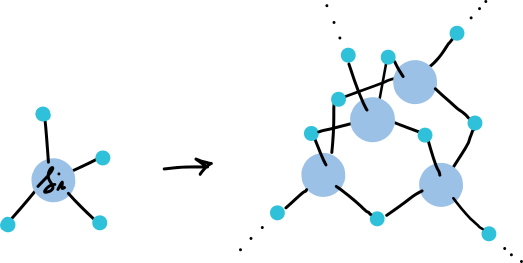
We established that Silicon doesn’t conduct electrons well because of its rigid tetrahedral structure, so how does a Silicon transistor conduct electrons? Well, the answer is \df{doping}—introducing a different set of atoms into the Silicon lattice to introduce either (1) valence shell openings through which electrons can flow or (2) excess electrons, which are loosely bound to the valence shell. Both of these methods increase conductivity throughout the lattice.

We introduce Boron atoms to create the valence shell openings mentioned in (1), which we refer to as \df{holes}. Boron has one less valence electron than Silicon, so when the predominantly Silicon tetrahedral lattice is formed, the Boron atom is left with one empty slot in its valence shell (see Figure \ref{#fig:P,N-type}{7}). This allows electrons to flow through the structure by jumping from hole to hole.

Another way to look at this is that the holes are moving through the lattice because once an electron jumps, one hole is opened and another is closed. When a hole moves to a Boron atom, an electron jumps from this Boron atom’s valence shell, increasing the charge of the Boron atom by +1. Therefore, we can say that these ‘positive’ holes move through the lattice. This is why we refer to this Silicon lattice doped with Boron as a \df{P-type} (positive-type) semiconductor—it conducts ‘positive’ holes.

On the other hand, we also create \df{N-type} (negative-type) semiconductors, by doping the Silicon lattice with Phosphorus, which has five valence electrons. Therefore, doping the Silicon lattice with Phosphorus introduces one extra electron for each added Phosphorus atom (recall that Silicon has 4 valence electrons).

When an electric field is applied to the lattice, these excess electrons accelerate in the direction of the field and create an electrical current, thereby increasing conductivity. So negative electrons flow through the N-type semiconductors, hence the name N-type.

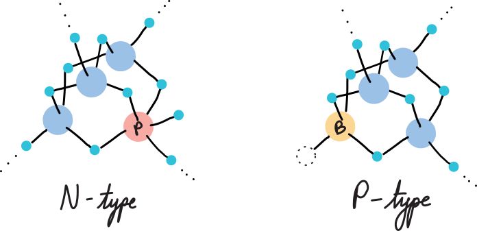
It’s easy to mistake the N/P-type naming convention for the semiconductors having either a negative or positive charge; however, both semiconductors are neutral in charge because the number of protons in the lattice’s nuclei equals the number of electrons in their valence shells. The naming convention refers to the types of charges that pass through the semiconductor: either positive holes (P-type) or negative electrons (N-type).

These two types of semiconductors make up the body of the transistor. Figure \ref{#fig:transistor}{8} gives a side-view of the transistor and the separation of N-type regions from the P-type region. Remember how the N-type semiconductors have one extra electron for each Phosphorus atom? This electron fills the holes of adjacent P-type semiconductors, introducing a negative charge to the originally neutral P-type semiconductor, thereby creating a negative barrier called the \df{depletion layer}.

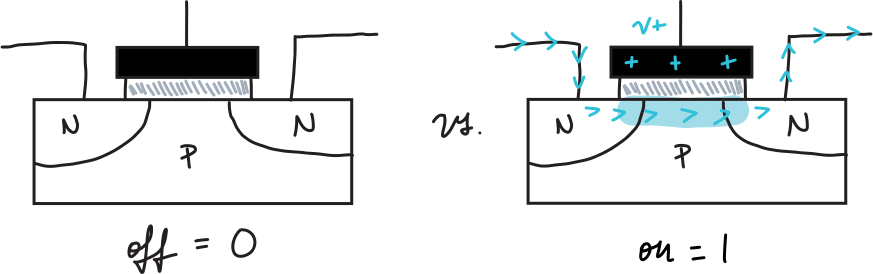
Electrons cannot pass this depletion layer without some help—think of when you try to press two magnets together on the same pole. However, by introducing a positive voltage in the gate of the transistor, the negative charge is effectively cancelled out, allowing electrons to flow freely from the left N-type semiconductor to the right one.

You may notice in the figure that there is a grey rectangle between the transistor’s gate and the semiconductors. This is the oxide layer, typically made of silicon dioxide, which insulates the gate just enough to prevent voltage from reaching the \df{substrate} of the transistor and affecting other transistors—the substrate is simply the floor of the microchip on which the transistor rests.

Manufacturing Transistors

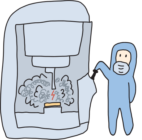
Microchip features are now on the scale of tens of nanometers (billionths of a meter)!⁶ When you hear that your computer’s microchip is a 5 nm process, this doesn’t refer to the size of the transistor, but rather the smallest feature that they can create using their manufacturing process. It used to be that transistor gate size correlated to process node naming, but that is no longer the case because certain parts are harder to scale down than others.

To manufacture such small features on microchips we use ultraviolet light pattern imprinting, also known as \df{lithography}, to etch features into the chip substrate. This involves putting various masks onto an intense UV light source which results in the pattern being transferred onto the chip.

Furthermore, various metals must be added onto the surface of the chip as a thin film to conduct electrons between various parts of the chip. One way to accomplish this is \df{Physical Vapor Deposition (PVD)} which involves heating a material in a vaccuum chamber until it evaporates and condenses onto the chip’s substrate. \df{Chemical Vapor Deposition (CVD)} is similar in that two gasses chemically react to form the thin film on the susbstrate.

This glimpse into chip manufacturing only scrapes the surface of the entire process, but hopefully it unveils some of the mystery regarding how these microchips are made. We now know how transistors work, the design philosophy behind them, and that they can store a binary state of 0 or 1. In the next section we’ll learn how to go from transistors simply holding state to creating a computer that can solve complex problems.

---

1. The word “bits” is a portmanteau—a blending of multiple words into one. In this case, we blend the words binary and digits: “binary”+“digits”\rightarrow “bits”.↩︎

2. This definition of functional completeness is not exactly correct as it does not pertain to boolean statements; however, we will refine this definition later on when we cover boolean algebra.↩︎

3. It also becomes harder to memorize all of these unique characters!↩︎

4. Another fun note on counting, if you’ve played piano, then you know that in an octave (e.g. C4 to C5) there are 12 half steps or equivalently 12 piano keys. In this way, the musical notes in all Western music is base-12!↩︎

5. The Greek etymology of tetrahedral: tetra “four” + hedra “face”.↩︎

6. For reference, the length of a human hair is 100 μm (micro-meters), or equivalently 100.000 nm.↩︎