Sets

Introduction

Set theory provides us with a basis of understanding for performing operations on big data, and performing these operations allow us to draw meaningful conclusions on the nature of the data. Having a solid understanding of set theory is imperative if you’re interested in becoming a data scientist.

Sets are simply groupings of distinct data points, and we mix and mash these sets together to draw conclusions about the data. Oftentimes, we perform these manipulations on data sets in SQL or Python’s pandas. For example, we may have an SQL database of real estate listings in a certain area and we want to find the listing which best fits the criteria that our investment company is interested in purchasing. Therefore, we take the set of all listings and apply a certain search criteria, which yields the set of listings that satisfy all of these criteria—in other words, the set defined by the overlapping criteria.

Figure \ref{#fig:david}{1} provides the illustrated analogy of Michelangelo carving away at a block of marble to make his statue of David, which is similar to the idea of applying criteria to a set to get rid of the unwanted data. It’s important to note that set operations also can be additive, meaning we add new elements to our set, but this drawing provides another way to view set theory.

Furthermore, if you’re interested in machine learning, then you’ll be happy to know that this section is important for you too. High quality data is integral to training efficient learning algorithms, and a strong foundation in set theory is essential for being able to work with and manipulate data.

What is a set?

Sometimes when people describe mathematical sets they use the analogy of a bag of items where any item is either in the bag or it isn’t, but there are no duplicate items in the bag. So if you had an apple in your bag and you placed another apple in the bag, you would still only have one apple in the bag. I find this definition to be rather confusing and improper as to what a set truly is.

When talking about sets I like to use the analogy of a person because every person is unique and special. Think of a list of adjectives you might use to describe yourself. Adjectives are simply umbrella terms for describing a collection of things that embody some common trait. For example, the adjective blonde means that you have yellowish hair, and this adjective encompasses all individuals with that hair color. In a sense, you belong to the group of individuals defined by the adjective blonde. You belong to many groups, but there is only one you. In the same way, an element may belong to many sets but there is only one element of that kind. Let’s say you are also tall, meaning you belong to the set of people denoted by the adjective ‘tall’. If we join the blonde set and the tall set of people together, thereby forming the set of people who are tall or blonde, we wouldn’t count you twice because there is only one you. Figure \ref{#fig:tall&blonde}{2} provides a graphic, Venn-diagram illustration of this idea.

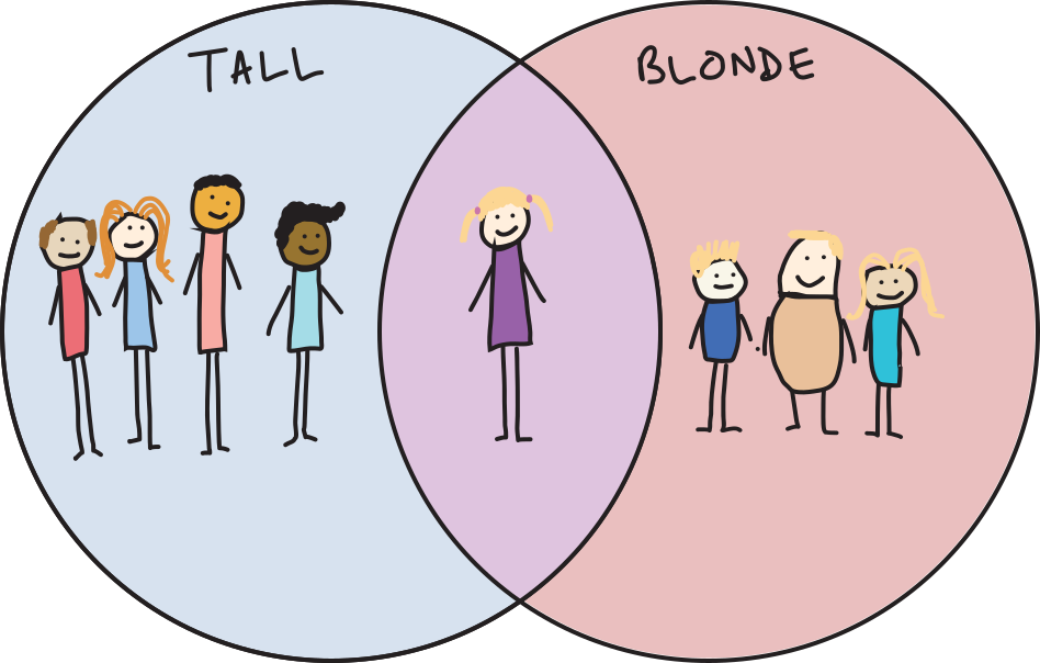
Therefore, a \df{set} is a group of distinct elements where the group is often defined by a membership criteria. In the analogy of blonde individuals, the set is the group of people with blonde hair, and the membership criteria is having blonde hair. The set answers the who and the membership criteria answers the why.

Sets can contain any number of elements, from no elements at all, to even an infinite number of elements—but usually we deal with finite sets. We refer to the set which contains no elements as the \df{empty set} which is notated as the symbol \emptyset. On the other hand, we refer to the set which contains every element as the \df{universal set}, notated as U.¹ We use the word \df{cardinality} to refer to the number of elements in a set, and we notate it using vertical bars. For example if set A has 3 elements, then we write |A|=3 and say, “A has a cardinality of 3”.

Set Construction

When denoting small finite sets, we use curly braces (e.g. \{1,2,3\}); however, for larger sets we use \df{set builder notation} which defines the set by the property or membership criteria its elements must satisfy. For example, we can notate the set of even numbers as \{x|\exists n\in\mathbb{Z}, x=2n\land x\ge 2\} which reads: “the set of all elements such that (1) for each element x there exists an integer n such that x=2n and (2) x is greater or equal to 2”. But sometimes it’s better to be lazy and you can simply write \{x|x \text{ is even and }x\ge 2\}. The key is remembering the idea that we are building a set by defining the membership property which every element in that set must satisfy.

We can also construct sets by taking the \df{Cartesian product} of two sets. For example, if I have the following sets: ranks=\{2,3,4,5,6,7,8,9,J,Q,K,A\} and suits=\{\heartsuit,\clubsuit,\spadesuit,\diamondsuit\}, we can form the set of all cards as ordered pairs of rank and suit by taking the Cartesian product, denoted by the symbol multiplication symbol: \eqlabel{Cartesian product}{1} cards = ranks\times suits=\{(2,\heartsuit),(2,\clubsuit),(2,\spadesuit),(2,\diamondsuit),(3,\heartsuit)\dots,(A,\diamondsuit)\}

Figure \ref{#fig:Cartesian visual}{3} provides an additional visual representation of the Cartesian product to help understand the operation better.

\begin{array}{r|cccc} & \heartsuit & \clubsuit & \spadesuit & \diamondsuit\\ \hline 2 & (2,\heartsuit) & (2,\clubsuit) & (2,\spadesuit) & (2,\diamondsuit)\\ 3 & (3,\heartsuit) & (3,\clubsuit) & (3,\spadesuit) & (3,\diamondsuit)\\ \vdots & \vdots & \vdots & \vdots & \vdots\\ A & (A,\heartsuit) & (A,\clubsuit) & (A,\spadesuit) & (A,\diamondsuit)\\ \end{array}

It’s important to note that the Cartesian product is not symmetric because it creates a set of ordered pairs. In equation \eqref{#Cartesian product}{1} if we were to reverse the order and say cards=suits\times ranks, we would produce a set of tuples where the order of each tuple is (suit,rank) rather than (rank,suit). Also, the cardinality of a Cartesian product of two sets is equal to the product of the cardinalities of its parent sets. So in the example of cards, |cards|=|rank|\cdot|suit|=13\cdot4=52.

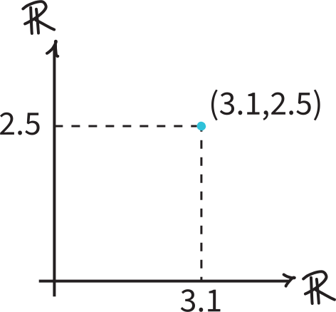
Here’s a quick connection to some of the math taught in high school. When we talk about coordinates in 2 dimensional space that contains all the points (x,y) we say that these points exist in \mathbb{R}^2, which is simply the space generated by the Cartesian product of the set of all reals multiplied by itself: denoted by \mathbb{R}\times\mathbb{R}=\mathbb{R}^2. See figure \ref{#fig:cartesian_plane}{4} for a visual example of the Cartesian product \mathbb{R}^2 as the plane containing ordered pairs of real numbers.

One last bit on Cartsian products and ordered pairs—sets do not inherently have order; however, we can map ordered pairs into the domain of sets using the following trick. We create a set of sets, such that given an ordered pair of n elements (b_1,b_2,\dots,b_n), we form a set containing n sets where the ith set contains all b_j such that 1\le j\le i. For example, (2,\heartsuit) maps to the set \{2,\{2,\heartsuit\}\}. We can write this mapping informally as

(b_1,b_2,\dots,b_n)\rightarrow \{b_1,\{b_j|1\le j\le 2\},\dots,\{b_j|1\le j\le n\}\}.

Another useful way to construct sets is through the use of powersets. Before we talk about powersets, we need to briefly define what a subset is. A \df{subset} is a set contained within a set. For example, if I have the set A=\{1,2,3\}, then B=\{1,2\} is a subset of A, denoted B\subseteq A. Any set is a subset of itself, and the empty set is a subset of every set.

A \df{powerset} is the set of all subsets of a given set. That’s a mouthful, but I promise it will make more sense once we look at an example. Let’s say we want to represent the set of all binary strings of length 3. Rather than writing out \{000,001,010,\dots,111\} or using set builder notation, \{x|b_2,b_1,b_0\in\{0,1\},x=b_2b_1b_0\}, we can also use powerset notation.

Let’s say we have the following set B=\{b_2,b_1,b_0\} where b_n is the nth bit in our binary string. We can define the set S=\{\emptyset,\{b_0\},\{b_1\},\{b_2\},\{b_1,b_0\},\{b_2,b_0\},\{b_2,b_1\},\{b_2,b_1,b_0\}\} such that each set in S maps to a binary string because the presence of a b_n in a set of S means that the nth bit of that binary string holds a value of 1. On the other hand, the absence of b_n in a set of S means that the nth bit holds a value of 0. S is the powerset of B, notated as P(B). Figure \ref{#fig:powerset}{5} provides the mapping of sets in P(B) to binary strings more clearly.

\begin{array}{l|l} \textbf{Subset} & \textbf{Binary String} \\ \hline \emptyset & 000\\ \{b_0\} & 001 \\ \{b_1\} & 010 \\ \{b_2\} & 100 \\ \hdashline \{b_1,b_0\} & 011 \\ \{b_2,b_0\} & 101 \\ \{b_2,b_1\} & 110 \\ \{b_2,b_1,b_0\} & 111 \\ \end{array}

This example of using powersets to create a mapping between sets and binary strings provides a great insight into the cardinality of powersets. Notice in figure \ref{#fig:powerset}{5} how each set in P(B) either includes each b_n of B or excludes it. So for each element of B there are 2 states as being included in a set or excluded. Since B has 3 elements, the total number of subsets of B is 2^3=8 by the product rule. Therefore, for any set A, |P(A)|=2^{|A|}.

Set Operations

Let’s take a look at some elementary set operations with the sets A=\{1,2\} and B=\{2,3\}.² Figure \ref{#fig:set ops}{6} shows these set operations as well as their English equivalents. Notice how in the union of A and B, the element 1 is not counted twice even though both sets contain 1. This is because the elements of a set are distinct, meaning you cannot have duplicates. Revisiting the person analogy for sets, if John is tall and likes fruit tart, then he belongs to both the set of people who are tall and the set of people who like fruit tart. Now if I take the union of those two sets, which includes people who are tall or like fruit tart, I don’t count John twice in the union because there is only one John.

operation	symbol	“elements in…”	result
complement	—	not A	\overline{A}=\{3\}
union	\cup	A or B.	A\cup B=\{1,2,3\}
intersect	\cap	A and B.	A\cap B=\{2\}
difference	\setminus	A and not B.	A\setminus B=\{1\}
symmetrical difference	\oplus	A or B but not both.	A\oplus B=\{1,3\}

Another helpful way to view these set operations is through their equivalent logical operators. Because sets are groups structured on membership—an element is either in the set or it isn’t—we can use a bit to represent each element’s membership in a certain set where 1 means the element is included and 0 means it is excluded. In this way, we create a bijection between the domain of sets and the codomain of binary strings.³ This translation between sets and bits is extremely powerful. Quickly returning to the adjective-person analogy for sets, we can create a binary ‘adjective vector’ such that each row of the vector is an adjective set and the value stored at that row is the person’s membership in that set. See figure \ref{#fig:set_vector}{7} for a visual representation of this.

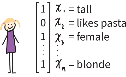
Figure \ref{#fig:binary sets}{8} which provides the binary string representation of sets A and B as well as the empty set and universal set.

Set	\mathbf{1}	\mathbf{2}	\mathbf{3}	Binary String
\emptyset	0	0	0	000
A=\{1,2\}	1	1	0	110
B=\{2,3\}	0	1	1	011
U=\{1,2,3\}	1	1	1	111

Now that we are working in the domain of bits, we can translate the set operations into their equivalent logical operations. Figure \ref{#fig:set logic ops}{9} provides the Boolean Algebraic expressions that correspond to each set operation. Notice how the English carries over directly into the Boolean operators.

set operation	“elements in…”	Boolean Algebra
\overline{A}=\{3\}	not A	\overline{110}=001
A\cup B=\{1,2,3\}	A or B	110+011=111
A\cap B=\{2\}	A and B	110\cdot 011=010
A\setminus B=\{1\}	A and not B	110\cdot\overline{011}=110\cdot 100=100
A\oplus B=\{1,3\}	A or B but not both	111\cdot\overline{010}=111\cdot101=101

Figure \ref{#fig:set logic ops}{9} provides a great transition into simplifying set expressions because it provides a translation from set theory to Boolean algebra, and we already know how to simplify Boolean algebraic expressions from chapter 1 section 2:s Boolean Algebra.

Simplifying Set Expressions

Recall DeMorgan’s law, which states that x\cdot y=\overline{\Bar{x}+\Bar{y}}. Because A\cap B is the set of all elements in A and B, by DeMorgan’s law it is equivalent to the set of all elements excluded from the set of elements not in A or not in B, which is \overline{\overline{A}\cup\overline{B}}. The set difference A\setminus B is the set of elements in A and not B, which is equivalent to A\cap\overline{B}. And the symmetrical difference A\oplus B is the set of elements in A or B but not both, which is equivalent to (A\cup B)\cap(\overline{A\cap B}). Figure \ref{#fig:set identities}{10} provides these set identities in tabular form.

\begin{array}{r|l} \textbf{set operation} & \textbf{equivalent identity}\\\hline A\setminus B & A\cap\overline{B}\\ A\oplus B & (A\cup B)\cap(\overline{A\cap B})\\ \end{array}

The set operators distribute and simplify in the same manner as Boolean algebraic operators. And now that we have learned the set identities given in figure \ref{#fig:set identities}{10}, we are simply working with Boolean ands, ors, and nots—we already know how to do this from chapter 1. Let’s go through an example of simplifying a set expression using the many laws of Boolean algebra that we learned in chapter 1. Figure \ref{#fig:set simplify}{11} details the steps taken to simplify a rather lengthy set expression.

\begin{array}{r l l} & (A\cap \overline{A}) \cup(A \cap(\overline{A} \cup \overline{B})) \cup (B \cap \overline{A \cap B}) &\\ \equiv & \textcolor{blue}{\emptyset} \cup(A \cap(\overline{A} \cup \overline{B})) \cup (B \cap \overline{A \cap B}) & \text{identity}\\ \equiv & (A \cap(\overline{A} \cup \overline{B})) \cup (B \cap \overline{A \cap B}) & \text{identity}\\ \equiv & (A \cap(\textcolor{blue}{\overline{\overline{{\overline{A} \cup \overline{B}}}}})) \cup (B \cap \overline{A \cap B}) & \text{double negation} \\ \equiv & (A \cap(\textcolor{blue}{\overline{A\cap B}})) \cup (B \cap \overline{A \cap B}) & \text{DeMorgan} \\ \equiv & (A\cap(\overline{A\cap B}))\cup (B\cap \textcolor{blue}{(}\overline{A\cap B}\textcolor{blue}{)}) & \text{commutative}\\ \equiv & \textcolor{blue}{(A\cup B)}\cap(\overline{A\cap B}) & \text{distributive}\\ \equiv & \textcolor{blue}{A\oplus B} & \text{definition of set difference} \end{array}

Set Partitions

Knowledge of set partitions is an important aspect of working with data because we may want to partition our large set of data into smaller, more manageable subsets such that our partition methods don’t assign data points to multiple sets or leave data points unassigned to a set, thereby yielding an incomplete partition of data.

To fully understand partitions we need to tie in the idea of disjoint sets. Two sets A and B are \df{disjoint} if A\cap B=\emptyset. A sequence of sets A_1,A_2,\dots,A_n is \df{pairwise disjoint} if every pair of distinct sets in the sequence is disjoint: \forall i,j\in[1,n],i\not=j:A_i\cap A_j=\emptyset. Given a set A, the sequence of sets A_1,A_2,\dots A_n is a partition of A iff the following conditions are met:

- \forall i\in[1,n]:A_i\subseteq A

- \forall i\in[1,n]:A_i\not=\emptyset

- A_1,A_2,\dots A_n is pairwise disjoint

- A_1\cup A_2\cup\dots\cup A_n=A

I like to think of a set partition like slicing a pizza. Regardless of how you slice, every bit of pizza is part of exactly one slice. See figure \ref{#fig:pizza_partition}{12} for a visual representation of this analogy.

Relations and Functions: Working with Sets

Binary Relations

Properties of Relations

Functions

Composition

Proofs in Propositional Logic

Rules of Inference

Direct Proofs

Proof by Contradiction

Proof by Contrapositive

Proof by Cases

Algorithms

Loop Invariants and Convergence

Combinatorics

Counting Principles (Addition, Multiplication, and Division Principles) Permutations and Combinations (with and without Repetition) Pigeonhole Principle Binomial Coefficients and Pascal’s Triangle

Permutation and Combination

Discreet Probability

Discrete Probability and Probability Distributions

Discrete Probability Spaces Probability Mass Function (PMF) Cumulative Distribution Function (CDF) Expected Value and Variance of Discrete Random Variables

Number Theory

Divisibility and Prime Numbers Greatest Common Divisor (GCD) and Least Common Multiple (LCM) Modular Arithmetic Euler’s Totient Function

Number Systems and Logic

Binary, Octal, and Hexadecimal Number Systems Boolean Algebra and Logic Gates Logic Circuits and Truth Tables

Recursion and Induction

Recursive Definitions and Recurrence Relations Solving Recurrence Relations Mathematical Induction and Strong Induction

Applications of Discrete Mathematics

Cryptography and Encryption Error Detection and Correction Codes Network and Graph Algorithms

Algorithms and Complexity

Introduction to Algorithms Algorithm Analysis (Time and Space Complexity) Sorting Algorithms (Bubble Sort, Merge Sort, Quick Sort) Searching Algorithms (Binary Search, Linear Search) Introduction to NP-Completeness

---

1. In some contexts, it makes sense for the universal set to only contain elements, but in other contexts it can also contain other sets. Also, the universal set differs from problem to problem, for example when dealing with finite sets, the universal set is usually the union of every set given in the problem.↩︎

2. Just to clarify, the word elementary is used in the sense of ‘foundational’ rather than ‘this is simple and you should get it instantly’. I dislike explanation that use words like ‘obviously’ or ‘clearly’ because they come across as unnecessarily patronizing.↩︎

3. Recall that a bijection is a mapping where every element in the codomain has exactly one element in the domain which maps to it.↩︎