
Fundamental Algorithms
What is an Algorithm?
An \df{algorithm} is simply a procedure or set of instructions used to solve a problem. For the sake of analogy, consider the act of folding laundry. When folding laundry, you follow a procedure of folding each article of clothing in a certain manner based on the set of clothes it belongs to (e.g. T-shirts, pants, socks, etc.). We can think of this procedure as iterating over our set of clothes and performing a series of Boolean if-then checks to see which fold to use. The algorithm is the procedure we follow, and can be semantically represented using code. See algorithm \ref{#fig:laundry algo}{1}, which provides the \df{pseudocode}1 corresponding to an algorithm for folding laundry.
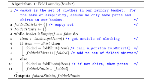
In algorithm \ref{#fig:laundry algo}{1}, we clearly define our input (basket) and our output (foldedShirts and foldedPants). The procedure is given in pseudocode with auxiliary comments to provide insight into what the code is doing. Algorithm \ref{#fig:laundry algo}{1} is an example of an \df{iterative algorithm} because the algorithm iterates over the elements of our input. We will touch more on the different classes of algorithms and problems later as we encounter them; however, in this section we will start at the fundamentals and build our way up.
Designing the Algorithm
Designing an algorithmic solution to a problem involves four key steps:
Consider the set of all possible inputs I. Identify the set of characteristics C which are found in every valid solution in our domain of possible solutions S given I: C=\bigcap_{s\in S} s.
Identify a generalized method for obtaining a solution that satisfies every c\in C.
Break this method down into a state machine representation of sequential steps such that each step handles every possible case we may encounter from the input. The Boolean checks in your state machine may contain vocabulary which carry along assumptions initially—this is ok!—but keep breaking these terms down and adding on more Boolean checks to discriminate between cases until every distinct case has a corresponding solution.2
Translate this state machine diagram into pseudocode, implementing all necessary data structures.
On the surface this formalized process of designing algorithms sounds complex, but we’ll see that it’s not as difficult as it may seem. Let’s try applying these four steps of designing an algorithm to the problem of folding laundry to understand how we obtained our pseudocode in algorithm \ref{#fig:laundry algo}{1}.
First we identify our set of all possible inputs I and set of solutions S that correspond to each input.
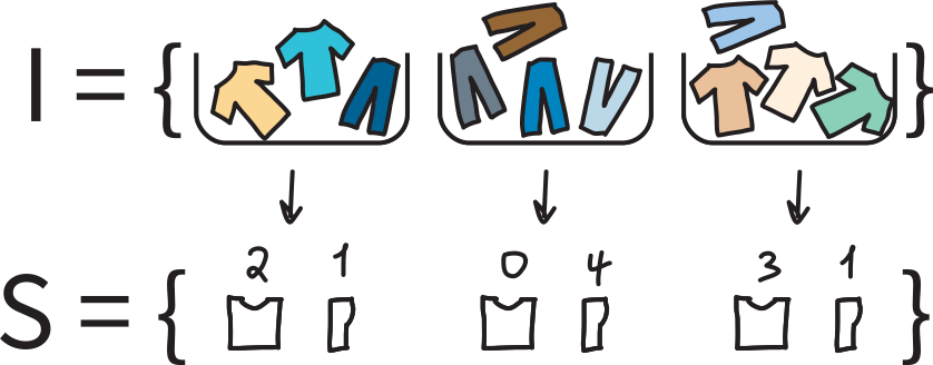
\figlabel{fig:C}{2} Set of all inputs I and set of all solutions S. We can quickly see that the set of characteristics common to our solutions C is defined as every article of clothing being grouped and folded according to its class—that being either a shirt or pants. Our solution should return the two sets of sorted clothes.3
The general method for obtaining a solution that satisfies our C is to fold fold everything according to its class and sort every folded item according to its class.
Figure \ref{#fig:state_laundry}{3} shows the state diagram representation of this generalized method. We first start with the big picture method, then we zoom in further to discriminate the articles of clothing by class.
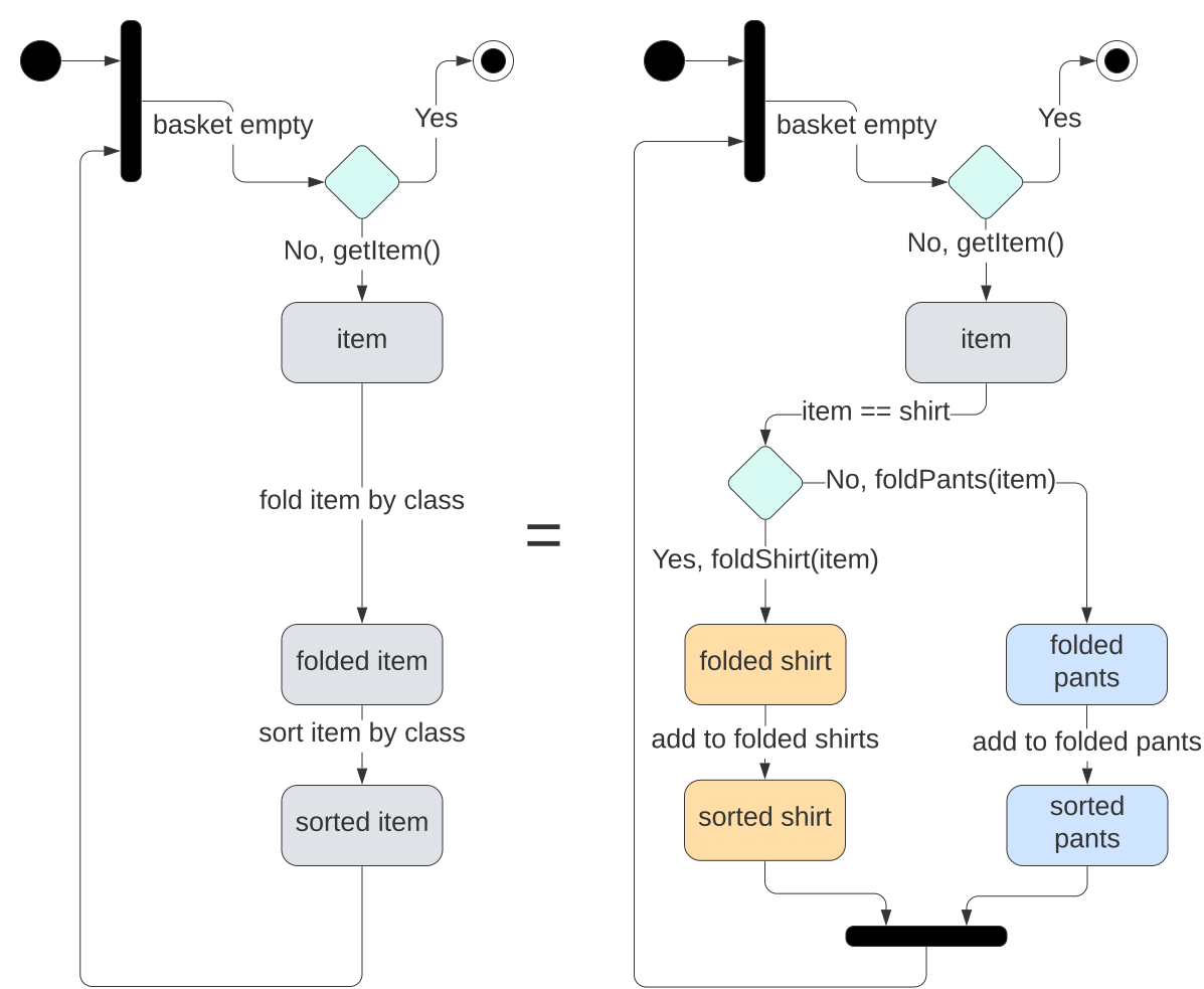
\figlabel{fig:state_laundry}{3} State diagrams for laundry folding algorithm. The diagram on left is high level and doesn’t consider the different classes of items. The diagram on the right provides a procedure which addresses all cases of item class and is therefore correct. We then obtain algorithm \ref{#fig:laundry algo}{1} from our state machine diagram in figure \ref{#fig:state_laundry}{3} by pairing the logic of our diagram with certain data structures.
It is important to note that invalid solutions to problems usually stem from an invalid handling of cases in step (3) due to an oversight of either certain cases or the incorrect grouping of two cases—thereby yielding a misclassification. For example, in the case of folding laundry, if our basket included both long-sleeve shirts and t-shirts, these would require different folding techniques. Therefore, we would need to modify algorithm \ref{#fig:laundry algo}{1} to differentiate between long-sleeve shirts and t-shirts.
The main takeaway from this section is that algorithms can be represented using state machine diagrams, which easily translate into code. By no means do you need to draw a state diagram every time you design an algorithm; however, keep this framework for developing algorithms in your toolkit. The best way to solve problems is to start from the big picture, then zoom in until you properly cover every possible edge case.
The Graph Data Structure
Remember in chapter 1 on bits how we talked about Leibniz’s discovery of counting in different bases? For example, we can represent the same number using base-10 (decimal), base-2 (binary), or base-16 (hexadecimal). In fact, we can use any base b\in\mathbb{Z}:b\ge 2 to represent a number.
The trade-off for choosing a certain b is that as we increase b we can store more information in each individual digit; however, to do so we need more unique single-element characters to represent each state of the digit (e.g. hexadecimal uses A-F for states 10-15). Computers represent information in binary because it tailors to the simple architecture of the transistor, which has two states.
In that same vein, when we represent information using a data structure there are many different options of data structures to choose from; however, we choose the data structure which most efficiently suits our needs for solving some problem.
A \df{graph} G=(V,E) is a data structure consisting of a set of n nodes V and a set of m edges E which connect these nodes. We represent an edge connecting node u and node v using the tuple (u,v). We can add features to our graph’s nodes and edges as needed to model problems (e.g. adding a table of edge weights W to our graph where W[(u,v)] is the distance from u to v). You will encounter graphs with directed edges (i.e. (u,v)\equiv u\rightarrow v \not\equiv v\rightarrow u); however, by default we assume that edges are bidirectional unless otherwise specified.
Let’s see how we can represent graphs using data structures that we’re already familiar with such as arrays and hash tables. Figure \ref{#fig:ex_graph}{4} provides a visualization of a (bidirectional) weighted graph.
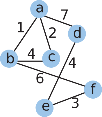
There are two main ways of representing G: (1) as an adjacency matrix or (2) as an adjacency list. Let’s see the difference and why we may opt for one or the other. An \df{adjacency matrix} is an n\times n matrix where the rows and columns represent nodes, and the entries of the matrix represent the presence of an edge. See figure \ref{#fig:adj_mat}{5} for the adjacency matrix of the graph from figure \ref{#fig:ex_graph}{4}.
Note that the graph from figure \ref{#fig:ex_graph}{4} is \df{connected}, which means that there is a path connecting any two nodes. However, if we were to add another node g to our graph in figure \ref{#fig:ex_graph}{4} such that g has no neighbors (i.e. no edges to other nodes), then the graph would no longer be connected. We would say that such a graph has two \df{connected components}, which are subgraphs that have the connected property. Think of the connected components in a graph as islands in an archipelago—if you’re walking on an island you can fully traverse it, but you cannot reach the other islands.4
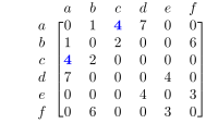
Now compare the adjacency matrix implementation from figure \ref{#fig:adj_mat}{5} with the equivalent representation of the graph using an adjacency list as shown in figure \ref{#fig:adj_list}{6}. Notice how we have less elements in our adjacency list data structure compared to the adjacency matrix because each row only contains neighbors rather than including zeros for non-neighbors as seen in the adjacency matrix.
\begin{array}{c|ccc} a & b & c & d\\ b & a & c & f\\ c & a & b &\\ d & a & e &\\ e & d & f &\\ f & b & e &\\ \end{array} \begin{array}{c|c} (a,b) & 1\\ (a,c) & 4 \\ (a,d) & 7 \\ (b,a) & 1\\ (b,c) & 2\\ (b,f) & 6\\ (c,a) & 4 \\ (c,b) & 2\\ (d,a) & 7 \\ (d,e) & 4 \\ (e,d) & 4 \\ (e,f) & 3 \\ (f,b) & 6\\ (f,e) & 3 \\ \end{array}
Now that we understand what a graph is and how to implement it using maps, let’s look at two ways of traversing our graph to obtain a \df{tree}, which is a connected graph without cycles. A \df{cylce} is simply a path or loop in the graph consisting of unique edges such that the starting node is also the ending node.
Graphs Traversal: BFS and DFS
There are two main ways to traverse a graph and obtain a tree: (1) Breadth First Search and (2) Depth First Search. For the sake of brevity, we refer to these as BFS and DFS, respectively. Both of these algorithms visit every node and edge in our graph G, and return a tree
Asymptotic Runtime
Graph Data Structures
Graph Isomorphism Graph Connectivity and Components Eulerian and Hamiltonian Paths and Circuits Trees and Binary Trees Spanning Trees
Min-Heap
Priority Queue
Tertiary Tree
Hashmaps
Dijkstra
Dynamic Programming
Mergesort
Knapsack, WIS, sequence aligning,
Network Flow
Ford-Fulkerson
Bellman-Ford
Capacity Scaling
Randomized Algorithms
Pseudocode is language-independent code, meaning that it uses English statements to convey the implementation of an algorithm rather using a specific coding language (e.g Python) to represent the algorithm.↩︎
The following paragraph will make this more clear when we apply these steps to the laundry folding problem.↩︎
In the case of folding clothes, identifying the characteristics of valid solutions is trivial; however, this step is important, especially when there are multiple valid solutions for each input.↩︎
For the sake of the analogy, assume there are no boats, helicopters, or planes to take you to the other islands.↩︎