Neural Networks
What are Thoughts?
Let’s take a closer look at how the brain works to understand the design philosophy behind neural networks.
As a fun example, let’s try visualizing a flamingo. Pause for a moment before reading on and think about what a flamingo looks like. Here’s what comes to my mind. A flamingo is pink, has a black tip on its beak, travels in large packs with other flamingos, and has tall nimble legs.
In order to generate that one thought we first looked at the ink on the page, decoded it into words and processed the meaning of each word while simultaneously processing the meaning of the sentence. Then we reached into our memory bank to recall everything related to flamingos. In other words, we took in visual data which activated different regions of our brain to abstract meaning from the data, and that meaning activated our memory recall to help us visualize flamingos.
Each region of your brain has billions of neurons which activate to different levels when you think and cause other neurons to activate.1 Let’s say that each neuron’s state lies in the continuous range from completely dormant, 0, to fully activated, 1. Stated formally, we say that neuron i has an activation
\eqlabel{eq:a_i}{1} a_i\in\mathbb{R}:a_i\in[0,1] Furthermore, each neuron is connected to other neurons, let’s call them neighbors, and the activation of one neuron affects the state of its neighbors.2
If I ask you the same question again, you’ll likely generate similar thoughts; however, these thoughts might differ from the first time I asked you. Therefore, something changed in your brain. The connectivity of certain neighboring neurons was either reduced or strengthened. We can say that each neural connection from neuron A to B has an associated connectivity scalar w_{AB} which changes the strength of the connection. If neuron i has n neighbors, borrowing the notation from equation \eqref{#eq:a_i}{1}, we can model its activation with
\eqlabel{eq:weight activation}{2} a_i\in\mathbb{R}:a_i\in[0,1]\land a_i=w_1a_1+w_2a_2+\ldots+w_na_n Therefore, neuron i’s activation a_i is a linear combination of its neighboring activations multiplied by their strength in connection to a_i. Right?—not quite.
We will see in the next section why this definition is incomplete, as well as how to fix it.
Linear Separability
In the previous section we came to the conclusion that a neuron’s activation is equal to a linear combination of its neighbors activations and connection strengths (see equation \eqref{#eq:weight activation}{2}). So how does this definition constrict the processing capabilities of our brain, considering that the brain is a network of neurons? Well the answer is linear separability.
Because we have defined every activation in our set of neurons to be a linear combination, we can only create thoughts which model linear relationships. In other words, our ability to separate two groups of data is limited to generating hyperplanes as our decision boundaries.
Recall that a hyperplane is a linear subspace with one less dimension than the space it occupies. For example a hyper plane in \mathbb{R}^2 is a one-dimensional line in \mathbb{R}. If we look at our expression for a_i from equation \eqref{#eq:weight activation}{2}, we can see that our linear combination of activations and weights is equivalent to the dot product of the weights and activations represented as vectors:
\eqlabel{eq:linear combo hyperplane}{3} a_i = w_1a_1+w_2a_2+\ldots+w_na_n = \begin{bmatrix} w_1 \\ w_2 \\ \vdots \\ w_n \end{bmatrix} \cdot \begin{bmatrix} a_1 \\ a_2 \\ \vdots \\ a_2 \end{bmatrix}= \mathbf{w_N}\cdot\mathbf{a_N}
If we take the gradient of our activation vector with respect to our weights \mathbf{w}—with respect to weights rather than activations because the weights or neural connection strengths are what we update, not activations—we get the dot product between a vector of 1s and our activations, causing our expression to evaluate to the sum of neihgboring activations, which is just a constant:
\eqlabel{eq:c=}{4} \begin{aligned} \nabla_\mathbf{w} a_i&= \nabla_\mathbf{w}(\mathbf{w_N} \cdot \mathbf{a_N}) =(\nabla_\mathbf{w}\mathbf{w_N})\cdot\mathbf{a_N}+\mathbf{w_N}\cdot(\nabla_\mathbf{w}\mathbf{a_N})\\ &= \begin{bmatrix} \pdv{w_1}{w_1}\\[0.5em] \pdv{w_2}{w_2}\\[0.5em] \vdots\\[0.5em] \pdv{w_n}{w_n} \end{bmatrix} \cdot \begin{bmatrix} a_1\\[0.5em] a_2\\[0.5em] \vdots\\[0.5em] a_n \end{bmatrix} + \begin{bmatrix} w_1 \\[0.5em] w_2\\[0.5em] \vdots\\[0.5em] w_n \end{bmatrix} \cdot \mathbf{0} = \begin{bmatrix} 1 \\ 1 \\ \vdots \\ 1 \end{bmatrix} \cdot \begin{bmatrix} a_1 \\ a_2 \\ \vdots \\ a_n \end{bmatrix} \\ &=a_1+a_2+\ldots+a_n=c:c\in\mathbb{R} \end{aligned}
Therefore, our variable a_i is bound to evaluate to a constant, thereby having one less degree of freedom than the dimension it occupies. Furthermore, because we know that the gradient evaluates to a constant, a_i is linear (i.e. its rate of change is constant). So we can say that a_i is a hyperplane.
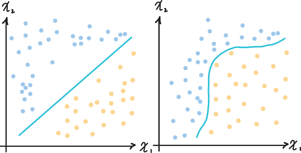
Figure \ref{#fig:linear sep}{1} shows the difference between linearly separable and non-linearly separable data. We can see that the decision boundary on the right in figure \ref{#fig:linear sep}{1} is clearly non-linear, and therefore not a hyperplane. So we cannot model non-linear systems with our current model of what a neuron is since our model only allows us to create hyperplanes.
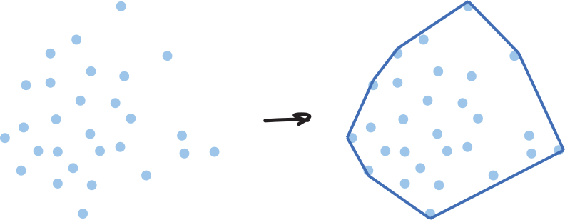
But how do we determine linear separability without drawing decision boundaries? Well, the answer is by drawing convex hulls. A convex hull is simply the smallest convex shape that can enclose all of our data points. Figure \ref{#fig:convex hull}{2} shows how to draw a convex hull from a set of data points in \mathbb{R}^2.
A dataset is linearly separable if there are two classes (we cannot separate a space into more than two subspaces using a single hyperplane) and the convex hulls of those two classes of points do not overlap. Figure \ref{#fig:convex overlap}{3} shows how the convex hulls of non-linear data overlap with each other.
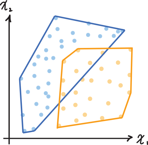
We now know that this model of the neuron is missing a component. Why? Because if you look at the non-linear data, your brain can visually generate the curved decision boundary separating the two classes—something that our model cannot do. Therefore, we need a non-linear component in our model of the neuron.
Rather than our activation a_i being determined by a linear combination of its n neighboring activations and weights, a_i is the output of a non-linear activation function g which takes in this linear combination as z_i and outputs a real number (see equation \eqref{#eq:preactivation and g}{5}).
\eqlabel{eq:preactivation and g}{5} \begin{aligned} z_i &=a_1w_1+a_2w_2+\ldots+a_nw_n= \begin{bmatrix} a_1 \\ a_2 \\ \vdots \\ a_n \end{bmatrix} \cdot \begin{bmatrix} w_1 \\ w_2 \\ \vdots \\ w_n \end{bmatrix}=\mathbf{a_N\cdot w_N}\\ a_i &=g(z_i)=g(\mathbf{a_N\cdot w_N}) \textit{ where $N=neighbors$.} \end{aligned}
Let’s recall the Taylor series, which allows us to model any infinitely differentiable function f(x) stationed at a using the power series formula
\eqlabel{Taylor Series}{6} T(x)=f(a)+\frac{f^{(1)}(a)}{1!}(x-a)+\frac{f^{(2)}(a)}{2!}(x-a)^2+\ldots+\frac{f^{(n)}(a)}{n!}(x-a)^n where f^{(n)}(a) is the nth derivative of f at a. Figure \ref{#fig:taylor series graph}{4} shows an example of Taylor expansion of f(x)=\sin x at a=0.
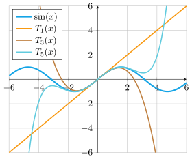
As n approaches infinity, the inaccuracies in our Taylor approximation T(x) iron out and the series approaches f(x) across the whole range of our domain x\in(-\infty,\infty).
Your brain’s network of neurons works in a similar way. Each neuron has a non-linear component g, and as an activation stimulus propagates (a fancy word for spreads) throughout the network it gets mushed and stretched by each neuron’s non-linear component to approximate some mapping of stimuli inputs to desired outputs.
The resulting data at the end is one that is linearly separable because we have created a non-linear decision boundary. For example in binary classification if we have generated the non-linear decision boundary d(x), our last layer of the network outputs a linear classifier l(x) which determines whether a point is below our decision boundary or above (see equation \eqref{#eq:linear classifier}{7}).
\eqlabel{eq:linear classifier}{7} l(x)= \begin{cases} 1 & \text{if $x\ge d(x)$} \\ 0 & \text{if $x<d(x)$} \end{cases}
Perceptrons: A Digital Analog to the Neuron
The perceptron is the fundamental building block of a neural network and it is similar to the brain’s neuron.
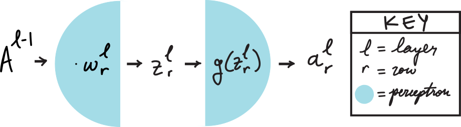
The perceptron consists of two parts, one linear and one non-linear. We call the first part linear because we perform a linear function. A perceptron in layer l and row r has an associated weight vector \mathbf{w_r^l}. We take the dot product of our input activation vector from the previous layer \mathbf{A^{l-1}}, where each element maps to a perceptron in the previous layer, and the perceptron’s weight vector \mathbf{w_r^l}:
\eqlabel{eq:linear half}{8} \mathbf{A^{l-1}}\cdot \mathbf{w_r^l}= \begin{bmatrix} a_1^{l-1} \\[0.5em] a_2^{l-1} \\[0.5em] \vdots \\[0.5em] a_m^{l-1} \end{bmatrix} \cdot \begin{bmatrix} w_{r1}^{l} \\[0.5em] w_{r2}^{l} \\[0.5em] \vdots \\[0.5em] w_{rm}^{l} \end{bmatrix} = a_1^{l-1}w_{r1}^l+a_2^{l-1}w_{r2}^l+\ldots+a_m^{l-1}w_{rm}^l = z_r^l
The second part is non-linear because we perform a non-linear activation function, denoted g(z). As we discussed in section 1.1, many relationships or mappings cannot be represented by a linear model alone. Therefore, we need to have the non-linear component in our perceptron to capture these non-linear relationships.
The function g takes z_r^l from equation (\ref{#eq:linear half}{8}) as input and applies a non-linear transformation:
\eqlabel{eq:nolinear_transformation}{9} g(z_r^l)=a_r^l
Figure \ref{#fig:perceptron}{5} shows this process of the perceptron transforming our input A^{l-1} into z_r^l in the linear part, then applying a on-linear transformation to this to obtain the activation vector for the next layer a_r^l.
Neural Network: A collection of Perceptrons
To create a neural network, we assemble a network of perceptrons organized into L layers where each of the n perceptrons in the current layer receives an activation vector A^{l-1} of m activations—one activation from each of the m perceptrons in the previous layer as shown in Figure \ref{#fig:NN}{6}.

For layer l we assemble every perceptron’s weight vector into the layer’s weight matrix W^l such that every column of W^l is a perceptron weight vector as shown in equation \eqref{#eq:W^l}{10}.
\eqlabel{eq:W^l}{10} W^l= \begin{bmatrix} \mathbf{w_1^l} & \mathbf{w_2^l} & \dots & \mathbf{w_n^l} \end{bmatrix} = \begin{bmatrix} w_{11}^l & w_{21}^l & \dots & w_{n1}^l \\ w_{12}^l & w_{22}^l & \dots & w_{n2}^l \\ \vdots & \vdots & \dots & \vdots \\ w_{1m}^l & w_{2m}^l & \dots & w_{nm}^l \end{bmatrix}
Recall the shape of activation vector A^{l-1} as shown in equation \eqref{#eq:bungus}{11}.
\eqlabel{eq:bungus}{11} \mathbf{A^{l-1}}= \begin{bmatrix} a_1^{l-1} \\[0.5em] a_2^{l-1} \\[0.5em] \vdots \\[0.5em] a_m^{l-1} \end{bmatrix}
To obtain our pre-activation vector \mathbf{Z^l} as a matrix multiplication of our weights and activations we must transpose our weight matrix, seen in equation \eqref{#eq:Z^l}{12}.
\eqlabel{eq:Z^l}{12} \begin{aligned} \mathbf{Z^l}= & (W^l)^T\mathbf{A^{l-1}}= \begin{bmatrix} w_{11}^l & w_{12}^l & \dots & w_{1m}^l \\[0.5em] w_{21}^l & w_{22}^l & \dots & w_{2m}^l \\[0.5em] \vdots & \vdots & \vdots & \vdots \\[0.5em] w_{n1}^l & w_{n2}^l & \dots & w_{nm}^l \end{bmatrix} \begin{bmatrix} a_1^{l-1} \\[0.5em] a_2^{l-1} \\[0.5em] \vdots \\[0.5em] a_m^{l-1} \end{bmatrix} \\ = & \begin{bmatrix} w_{11}^la_1^{l-1}+w_{12}^la_2^{l-1}+\dots+w_{1m}^la_m^{l-1} \\[0.5em] w_{21}^la_1^{l-1}+w_{22}^la_2^{l-1}+\dots+w_{2m}^la_m^{l-1} \\[0.5em] \vdots \\[0.5em] w_{n1}^la_1^{l-1}+w_{n2}^la_2^{l-1}+\dots+w_{nm}^la_m^{l-1} \end{bmatrix} = \begin{bmatrix} z_1^{l} \\[0.5em] z_2^{l} \\[0.5em] \vdots \\[0.5em] z_n^{l} \end{bmatrix} \end{aligned}
Equation \eqref{#eq:transpose algebra}{13} shows a dimensional analysis of the matrix multiplication to clearly show why we must take the transpose of W^l.
\eqlabel{eq:transpose algebra}{13} \begin{aligned} \mathbf{Z^l}&=(W^l)^T\mathbf{A^{l-1}}=(m\times n)^T\times(m\times1)=(n\times m)\times(m\times1) \\ &=(n\times m) \end{aligned}
We then apply our non-linear activation function g to each element in our preactivation vector Z^l to obtain our activation vector A^l as shown in equation \eqref{#eq:A^l}{14}, which we use for the next layer in our network.
\eqlabel{eq:A^l}{14} \mathbf{A^l}=g(\mathbf{Z^l})= \begin{bmatrix} g(z_1^{l}) \\[0.5em] g(z_2^{l}) \\[0.5em] \vdots \\[0.5em] g(z_n^{l}) \end{bmatrix}
Formal Definition of a Neural Network
Neural networks can initially appear to be magical black boxes that somehow do everything. They can draw like Picasso, play chess better than Magnus Carlsen, and code programs from simple word prompts. However, upon closer examination we realize that a neural network is simply a function \hat{y}=\mathcal{F}(x) that maps our domain to the codomain, \mathcal{F}:X\rightarrow Y. The network learns this mapping by training on a dataset which maps a subset of our domain to the codomain.
Formally, given a dataset of pairs \{x^{(i)},y^{(i)}\}, which is a partial mapping D:X\rightharpoonup Y, we define a loss function \mathcal{L}(\hat{y},y) representing the discrepancy between our network’s mapping \hat{y} and the mapping y from our dataset, and in each training iteration we update the network’s set of weights W to minimize this loss: \eqlabel{eq:W_new}{15} W_{new}=\argmin_W\mathcal{L}(\hat{y},y)=W_{old}-\alpha\nabla_W\mathcal{L}(\hat{y},y) Eventually the marginal decrease in our loss function \mathcal{L} approaches zero, at which point the network has converged and we have maximized the correspondence between the network’s mapping and the dataset’s partial mapping.
Non-linear Activation Functions
Let’s examine perceptron in layer l and row r of our network. We know that the perceptron needs a non-linear activation function g to modify the linear combination z_r^l=\mathbf{A^{l-1}\cdot w_r^l} (preactivation) in order order to form non-linear decision boundaries, but how do we choose a good g? Let’s recall our definition of a neuron’s activation a_i\in\mathbb{R}:a_i\in[0,1] which states that the activation lies somewhere in the range from 0 to 1. Therefore, we want our function g to bind our preactivation z to this range. Figure \ref{#fig:sigmoid}{7} shows the sigmoid activation function \sigma(z) (also known as the logistic function), which is bound by the horizontal asymptotes at y=0 and y=1. \sigma(z) approaches these asymptotes, but never takes on their value, so we can say that \sigma(z)\in\mathbb{R}:\sigma(z)\in(0,1).
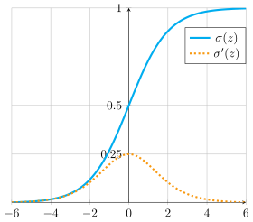
Notice how \sigma(z) looks linear as we get closer to z=0. It looks like the line y=0.25z+0.5, which we can verify by looking at the derivative of the sigmoid, \sigma'(z), which is plotted in orange dots in the same figure. We can verify this by looking at figure \ref{#fig:sigmoid}{7} and which shows the sigmoid’s derivative \sigma'(z) having a value of 0.25 at z=0. The sigmoid function is monotonic increasing, meaning as z increases, \sigma(z) either increases or remains constant, but never decreases. It is also differentiable across the whole domain. However, one drawback is that it is computationally expensive to calculate due to there being an exponent in the expression (recall that the function is \sigma(z)=\frac{1}{1+e^{-z}}).
Furthermore, we may face the vanishing gradient problem during backpropagation, where the gradient of our loss function with respect to each weight becomes so small that we cannot .